Workflow diagram

Analysis using GeoAnalytics Tools

Analysis using GeoAnalytics Tools is run using distributed processing across multiple ArcGIS GeoAnalytics Server machines and cores. GeoAnalytics Tools and standard feature analysis tools in ArcGIS Enterprise have different parameters and capabilities. To learn more about these differences, see Feature analysis tool differences.

Terminology

Examples

Hurricanes are some of the most violent types of storms that occur in the United States. To assess insurance rates, you want to know the paths that hurricanes have traveled to determine locations that have historically had high property damage and financial loss from hurricanes. You have access to hurricane location data across the United States in a single dataset, with a timestamp at each location. You want to summarize all the information to see a summary of values for all hurricanes. You can summarize your data using the hurricane tracks identifier to determine the statistics for each hurricane.

Usage notes

Reconstruct Tracks is run on point or area features. The input layer must be time enabled with features that represent an instant in time.

For linear results, only tracks that contain more than one point will be returned. If you apply a buffer, all features will be returned.

Input features will consist of time-enabled features that represent an instant in time. Results are line or area features that represent an interval in time. The start and end of the interval are determined by the time at the first and last features in a track.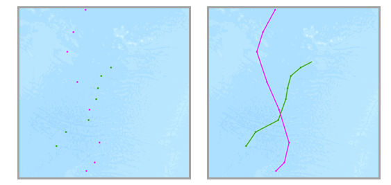

The most basic calculation in a track will be a count of the number of features that have been summarized. Statistics (count, sum, minimum, maximum, range, mean, standard deviation, and variance) can also be calculated on numerical fields, and statistics (count and any) can be calculated on string fields. The string statistic any returns a sample string from each track. The statistics will be calculated on each track separately.

The field or fields used to identify tracks will be returned in the results.

You can specify one or more fields to identify tracks. Tracks are represented by the unique combination of one or more track fields. For example, if the fields flightID and Destination are used as track identifiers, the features ID007, Solden and ID007, Tokoyo would be in two separate tracks, since they have different Destination field values.

You can optionally apply a buffer to your input features. When you apply a buffer, resulting tracks will be area features.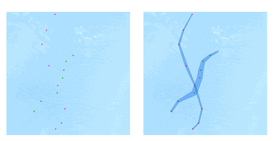

Buffers are created using a field or a buffer expression. To learn more about buffer expressions and formatting, see Use buffer expressions with GeoAnalytics Tools. You can apply a track-aware expression. For example, you could buffer the current feature by the mean of the field wind_speed for the previous three features in a track with the equation mean($track.field["wind_speed].history(-4, -1)).

When buffering input features, each input feature is buffered. Then a convex hull is generated to create an area track.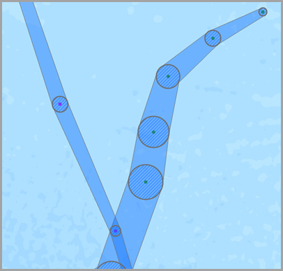

By default, tracks are created using a geodesic method. The method is applied to the following two components of the analysis:

• Tracks crossing the international date line—When using the geodesic method, input layers that cross the international date line will have tracks that correctly cross the international date line. This is the default. Your input layer or processing spatial reference must be set to a spatial reference that supports wrapping around the international date line, such as a global projection like World Cylindrical Equal Area.
• Buffers—Input features can optionally be buffered. To learn more about when to apply a geodesic or planar buffer, see Create buffers.

There are three ways to split tracks:

• Based on a time between inputs—Applies a time split
• At defined time intervals—Applies a time boundary
• Based on a distance between inputs—Applies a distance split

Applying a time split breaks any track apart when input data is further apart than the specified time. For example, if you had five features with the same track identifier and the times of [01:00, 02:00, 03:30, 06:00, 06:30] and set a time split of two hours, any features that are measured more than two hours apart will be split. In this example, the result would be a track with [01:00, 02:00, 03:30] and [06:00, 06:30], because the difference between 03:30 and 6:00 is greater than two hours.

Applying a time boundary segments tracks at a defined interval. For example, if you set the time boundary to be 1 day, starting at 9:00 AM on January 1, 1990, each track will be truncated at 9:00 AM for every day. This split is a fast way to accelerate computing time, as it quickly creates smaller tracks for analysis. If splitting by a recurring time boundary makes sense for your analysis, it is recommend for big data processing.

Applying a distance split breaks any track apart when input data is further apart than the specified distance. For example, if you set a distance split of 5 kilometers and sequential features greater than 5 kilometers apart would be part of a different track.

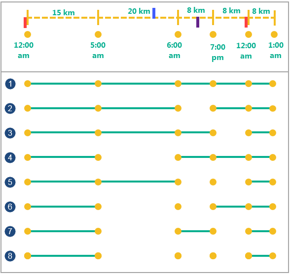
You can apply none, one, two, or three split options at the same time. The different results, assuming we apply a time split of 6 hours, a time boundary of 1 day, and distance split of 16 kilometers would be as follows:

Split option	Description
Six input points with a time and location.	Input points with the same identifier. The distance between the points is marked on the top of the dotted line, and the time of each point measurement is marked below the points. There are four splits on the timeline. The red splits represent the time boundary split of 1 day, starting at 12:00 AM. The blue split represents the distance split, when the distance between two points is greater than 16 km. The purple split represents the time split, when the temporal distance between two sequential points is greater than 6 hours.
	Example with no time split and no distance split.
	Example with a time split of two hours. Any features greater than two hours apart are split into separate tracks.
	Example with a time boundary of 1 day, starting at midnight. At each 1-day interval starting from the specified time (here 12:00 AM), a new track is created..
	Example with a distance split of 16 kilometers. Any features greater than 16 kilometers apart (the features at 05:00 AM and 06:00 AM) are split into separate tracks.
	Example with a time split of 6 hours and a time boundary of 1 day starting at 12:00 AM. Any features greater than six hours apart or that intersect with the time duration split at 12:00 AM are split into separate tracks.
	Example with a time split of 6 hours and a distance split of 16 km. Any features greater than six hours apart (the features at 06:00 AM and 7:00 PM) or farther than 16 km apart are split into separate tracks.
	Example with a distance split of 16 km and a time boundary of one starting at 12:00 AM. Any features greater than 16 km apart or that intersect with the time duration split at 12:00 AM are split into separate tracks.
	Example with a distance split of 16 km, a time split of 6 hours, and a time boundary of one day starting at 12:00 AM. Any features greater than 16 km apart, or farther apart than 6 hours, or that intersect with the time duration split at 12:00 AM are split into separate tracks.

The following are examples of how it might make sense to define tracks using the split parameters and the field identifier parameter using an airline flight as an example:

• An aircraft feature has aircraft ID, flight ID, pilot name, and start time fields.
  • Use the aircraft ID as the identifier if you are interested in seeing where each plane has traveled.
  • Use the aircraft ID and the flight ID field as the identifier if you are interested in comparing distinct routes.
  • Use the aircraft id and the time boundary of 1 year, if you want to examine the flights for each aircraft for a year at a time.
  • Use the pilot name, aircraft ID, and start time if you want to look at each pilots' flight.
  • Use the aircraft ID as the identifier, and split on distances greater than 1000 kilometers to determine new tracks, given that a 1,000-kilometer jump in measurements should not belong to the same track. .

Output tracks will return the fields used as track identifiers, the count of features within a track (count), the start and end time of each track (start_datetime and end_datetime), the duration of the track in milliseconds (duration) and any other optional statistics.

If Use current map extent is checked, only the features that are visible within the current map extent will be analyzed. If it's not checked, all input features in the input layer will be analyzed, even if they are outside the current map extent.

Limitations

Inputs must be point or area layers with time enabled features of type instant. Any features that do not have time will not be included in the output tracks.

How Reconstruct Tracks works

Equations

Variance is calculated using the following equation: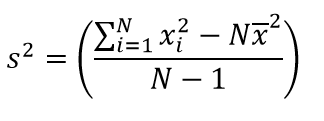

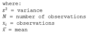
Standard deviation is calculated as the square root of the variance.

ArcGIS API for Python example

The Reconstruct Tracks tool is available through ArcGIS API for Python.

# Import the required ArcGIS API for Python modules
import arcgis
from arcgis.gis import GIS
from arcgis.geoanalytics import summarize_data

# Connect to your ArcGIS Enterprise portal and check that GeoAnalytics is supported
portal = GIS("https://myportal.domain.com/portal", "gis_publisher", "my_password", verify_cert=False)
if not portal.geoanalytics.is_supported():
    print("Quitting, GeoAnalytics is not supported")
    exit(1)   

# Find the big data file share dataset you're interested in using for analysis
search_result = portal.content.search("", "Big Data File Share")

# Look through search results for a big data file share with the matching name
bd_file = next(x for x in search_result if x.title == "bigDataFileShares_NaturalDisasters")

# Look through the big data file share for hurricanes
hurricanes = next(x for x in bd_file.layers if x.properties.name == "Hurricanes")

# Set the tool environment settings
arcgis.env.verbose = True

# Reconstruct the hurricane tracks by their serial_number 
track_result = summarize_data.reconstruct_tracks(input_layer = hurricanes, 
                                                 track_fields = "serial_num",
                                                 method = 'Geodesic',
                                                 output_name = "hurricane_tracks")

# Visualize the tool results if you are running Python in a Jupyter Notebook
processed_map = portal.map('World')
processed_map.add_layer(track_result)
processed_map

Similar tools

Use Reconstruct Tracks to summarize features within a track. Other tools may be useful in solving similar but slightly different problems.